Lateral earth pressure is the pressure that soil exerts in the horizontal direction. The lateral earth pressure is important because it affects the consolidation behavior and strength of the soil and because it is considered in the design of geotechnical engineering structures such as retaining walls, basements, tunnels, deep foundations and braced excavations.
The coefficient of lateral earth pressure, K, is defined as the ratio of the horizontaleffective stress, σ’h, to the vertical effective stress, σ’v. The effective stress is the intergranular stress calculated by subtracting the pore pressure from the total stress as described in soil mechanics. K for a particular soil deposit is a function of the soil properties and the stress history. The minimum stable value of K is called the active earth pressure coefficient, Ka; the active earth pressure is obtained, for example,when a retaining wall moves away from the soil. The maximum stable value of K is called the passive earth pressure coefficient, Kp; the passive earth pressure would develop, for example against a vertical plow that is pushing soil horizontally. For a level ground deposit with zero lateral strain in the soil, the "at-rest" coefficient of lateral earth pressure, K0 is obtained.
There are many theories for predicting lateral earth pressure; some are empirically based, and some are analytically derived.
Contents
- 1 At rest pressure
- 2 Soil Lateral Active Pressure and Passive Resistance
- 2.1 Rankine theory
- 2.2 Coulomb theory
- 2.3 Caquot and Kerisel
- 2.4 Equivalent fluid pressure
- 3 Bell's relationship
- 4 Coefficients of earth pressure
At rest pressure
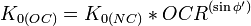
At rest lateral earth pressure, represented as K0, is the in situ lateral pressure. It can be measured directly by a dilatometertest (DMT) or a borehole pressuremeter test (PMT). As these are rather expensive tests, empirical relations have been created in order to predict at rest pressure with less involved soil testing, and relate to the angle of shearing resistance. Two of the more commonly used are presented below.Jaky (1948) for normally consolidated soils:Mayne & Kulhawy (1982) for overconsolidated soils:The latter requires the OCR profile with depth to be determined. OCR is the overconsolidation ratio and is the effective stress friction angle.To estimate K0 due to compaction pressures, refer Ingold (1979)
Soil Lateral Active Pressure and Passive Resistance
The active state occurs when a retained soil mass is allowed to relax or deform laterally and outward (away from the soil mass) to the point of mobilizing its available full shear resistance (or engaged its shear strength) in trying to resist lateral deformation. That is, the soil is at the point of incipient failure by shearing due to unloading in the lateral direction. It is the minimum theoretical lateral pressure that a given soil mass will exert on a retaining that will move or rotate away from the soil until the soil active state is reached (not necessarily the actual in-service lateral pressure on walls that do not move when subjected to soil lateral pressures higher than the active pressure). The passive state occurs when a soil mass is externally forced laterally and inward (towards the soil mass) to the point of mobilizing its available full shear resistance in trying to resist further lateral deformation. That is, the soil mass is at the point of incipient failure by shearing due to loading in the lateral direction. It is the maximum lateral resistance that a given soil mass can offer to a retaining wall that is being pushed towards the soil mass. That is, the soil is at the point of incipient failure by shearing, but this time due to loading in the lateral direction. Thus active pressure and passive resistance define the minimum lateral pressure and the maximum lateral resistance possible from a give mass of soil.Rankine theory
Rankine's theory, developed in 1857, is a stress field solution that predicts active and passive earth pressure. It assumes that the soil is cohesionless, the wall is frictionless, the soil-wall interface is vertical, the failure surface on which the soil moves is planar, and the resultant force is angled parallel to the backfill surface. The equations for active and passive lateral earth pressure coefficients are given below. Note that φ' is the angle of shearing resistance of the soil and the backfill is inclined at angle β to the horizontalFor the case where β is 0, the above equations simplify toCoulomb theory
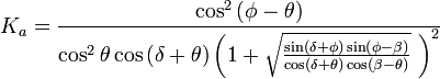
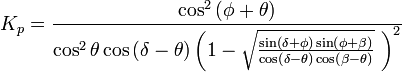
Coulomb (1776) first studied the problem of lateral earth pressures on retaining structures. He used limit equilibrium theory, which considers the failing soil block as a free body in order to determine the limiting horizontal earth pressure. The limiting horizontal pressures at failure in extension or compression are used to determine the Ka and Kp respectively. Since the problem is indeterminate,a number of potential failure surfaces must be analysed to identify the critical failure surface (i.e. the surface that produces the maximum or minimum thrust on the wall). Mayniel (1908) later extended Coulomb's equations to account for wall friction, symbolized by δ. Müller-Breslau (1906) further generalized Mayniel's equations for a non-horizontal backfill and a non-vertical soil-wall interface (represented by angle θ from the vertical).Instead of evaluating the above equations or using commercial software applications for this, books of tables for the most common cases can be used. Generally instead of Ka, the horizontal part Kah is tabulated. It is the same as Ka times cos(δ+θ).The actual earth pressure force Ea is the sum of a part Eag due to the weight of the earth, a part Eap due to extra loads such as traffic, minus a part Eac due to any cohesion present.Eag is the integral of the pressure over the height of the wall, which equates to Ka times the specific gravity of the earth, times one half the wall height squared.In the case of a uniform pressure loading on a terrace above a retaining wall, Eap equates to this pressure times Ka times the height of the wall. This applies if the terrace is horizontal or the wall vertical. Otherwise, Eap must be multiplied by cosθ cosβ / cos(θ − β).Eac is generally assumed to be zero unless a value of cohesion can be maintained permanently.Eag acts on the wall's surface at one third of its height from the bottom and at an angle δ relative to a right angle at the wall. Eap acts at the same angle, but at one half the height.