The cobweb model or cobweb theory is an economic model that explains why prices might be subject to periodic fluctuations in certain types of markets. It describes cyclical supply and demand in a market where the amount produced must be chosen before prices are observed. Producers' expectations about prices are assumed to be based on observations of previous prices. Nicholas Kaldor analyzed the model in 1934, coining the term 'cobweb theorem' (see Kaldor, 1938 and Pashigian, 2008), citing previous analyses in German by Henry Schultz and Umberto Ricci (it).
Contents
- 1 The model
- 2 Elasticities versus slopes
- 3 Role of expectations
- 4 Evidence
- 4.1 Livestock herds
- 4.2 Human experimental data
- 4.3 Housing Sector in Israel
The model
.svg)
.svg)
The cobweb model is based on a time lag between supply and demand decisions. Agricultural markets are a context where the cobweb model might apply, since there is a lag between planting and harvesting (Kaldor, 1934, p. 133-134 gives two agricultural examples: rubber and corn). Suppose for example that as a result of unexpectedly bad weather, farmers go to market with an unusually small crop of strawberries. This shortage, equivalent to a leftward shift in the market's supply curve, results in high prices. If farmers expect these high price conditions to continue, then in the following year, they will raise their production of strawberries relative to other crops. Therefore when they go to market the supply will be high, resulting in low prices. If they then expect low prices to continue, they will decrease their production of strawberries for the next year, resulting in high prices again.
This process is illustrated by the diagrams on the right. The equilibrium price is at the intersection of the supply and demand curves. A poor harvest in period 1 means supply falls to Q1, so that prices rise to P1. If producers plan their period 2 production under the expectation that this high price will continue, then the period 2 supply will be higher, at Q2. Prices therefore fall to P2 when they try to sell all their output. As this process repeats itself, oscillating between periods of low supply with high prices and then high supply with low prices, the price and quantity trace out a spiral. They may spiral inwards, as in the top figure, in which case the economy converges to the equilibrium where supply and demand cross; or they may spiral outwards, with the fluctuations increasing in magnitude.
Simplifying, the cobweb model can have two main types of outcomes:
- If the supply curve is steeper than the demand curve, then the fluctuations decrease in magnitude with each cycle, so a plot of the prices and quantities over time would look like an inward spiral, as shown in the first diagram. This is called the stable or convergent case.
- If the slope of the supply curve is less than the absolute value of the slope of the demand curve, then the fluctuations increase in magnitude with each cycle, so that prices and quantities spiral outwards. This is called the unstable or divergent case.
Two other possibilities are:
- Fluctuations may also remain of constant magnitude, so a plot of the outcomes would produce a simple rectangle, if the supply and demand curves have exactly the same slope (in absolute value).
- If the supply curve is less steep than the demand curve near the point where the two curves cross, but more steep when we move sufficiently far away, then prices and quantities will spiral away from the equilibrium price but will not diverge indefinitely; instead, they may converge to a limit cycle.
In either of the first two scenarios, the combination of the spiral and the supply and demand curves often looks like a cobweb, hence the name of the theory.
Elasticities versus slopes
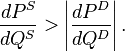
The outcomes of the cobweb model are stated above in terms of slopes, but they are more commonly described in terms of elasticities. In terms of slopes, the convergent case requires that the slope of the supply curve be greater than the absolute value of the slope of the demand curve:
In standard terminology from microeconomics, define the elasticity of supply as  , and the elasticity of demand as
  . If we evaluate these two elasticities at the equilibrium point, that is
  and
and  , then we see that the convergent case requires
, and the elasticity of demand as . If we evaluate these two elasticities at the equilibrium point, that is and , then we see that the convergent case requires
whereas the divergent case requires

In words, the convergent case occurs when the demand curve is more elastic than the supply curve, at the equilibrium point. The divergent case occurs when the supply curve is more elastic than the demand curve, at the equilibrium point (see Kaldor, 1934, page 135, propositions (i) and (ii).)